11 Expected Utility

In decision-making under uncertainty, evaluating and comparing lotteries requires more than just knowing a decision maker’s preferences over outcomes. Expected utility provides a systematic way of assigning a single utility value to each lottery, based on the probabilities of different outcomes and the utilities associated with them. Before diving into expected utility, it’s helpful to first understand the concept of expected value.

When the prizes are monetary values, a decision maker can compare lotteries using the expected value of the lottery.

Definition 11.1 (Expected value) Suppose that $L = p_1 \cdot x_1 + \cdots + p_n \cdot x_n$ is a lottery where, for each $i = 1, \ldots, n$, the outcome $x_i$ represents an amount of money. The expected value of $L$ is defined as: \[EV(L)=\sum_{i=1}^n p_i \times x_i.\]

For example, if $L = 0.5 \cdot \$100 + 0.5 \cdot \$0$, then $EV(L) = 0.5 \times 100 + 0.5 \times 0 = 50$. This means that, on average, you would expect to receive $\$50$ from this lottery. To illustrate this concept, the following simulation shows the average payout after playing this lottery $1,000$ times (you can experiment by changing the probabilities and payouts).

viewof p = Inputs.form({
  prize1: Inputs.range([0, 100], {step: 1, value: 100, label: "prize 1"}),
  prize2: Inputs.range([0, 100], {step: 1, value: 0, label: "prize 2"}),
  prob: Inputs.range([0, 1], {step: 0.01, value:0.5, label: "probability of prize 1"}),
})

tex.block`
  EV(${p.prob} \cdot ${p.prize1} + ${Math.round((1-p.prob)*100) / 100} \cdot ${p.prize2})  = ${p.prob} \times ${p.prize1} + ${Math.round((1-p.prob)*100) / 100} \times ${p.prize2} = ${Math.round((p.prob * p.prize1 + (1-p.prob) * p.prize2) *1000) / 1000}
`

data_ev={
  let p1_data = {prize: "$" + p.prize1.toString(), num: 0};
  let p2_data = {prize: "$" + p.prize2.toString(), num: 0};
  let x = 0;
  for (let i = 0; i < 1000; i++) {

    let outcome = Math.random() < p.prob ? 1 : 0;
    p1_data["num"] += outcome;
    p2_data["num"] += 1-outcome;
    
}
  return [p1_data, p2_data];
}

md`After playing the lottery 1,000 times, the average payout is **${(data_ev[0]["num"] * p.prize1 + data_ev[1]["num"] * p.prize2) / 1000}**. The number of times each prize was won is given in the following bar graph: `

Plot.plot({
  marks: [
    Plot.barY(data_ev, {x: "prize", y: "num"}),
    Plot.text(data_ev, {x: "prize", y: "num", text: d => d.num, dy: -10}) // Adding labels to the bars
  ]
})

Comparing lotteries by expected value means that a decision maker strictly prefers $L$ to $L'$ if $EV(L) > EV(L')$. In this case, the decision maker would choose $L$ over $L'$ when the expected value of $L$ is greater than that of $L'$. Consequently, a decision maker would be willing to pay up to $EV(L)$ in exchange for playing the lottery $L$.

While expected value provides a straightforward method for evaluating lotteries, it often falls short in addressing the complexities of real-world decision-making, even when the outcomes involve monetary amounts. Several factors contribute to why we cannot rely solely on expected value:

Valuing Money: The value of a wager depends on more than just its expected payout. Individual factors, such as your total wealth, how much you personally value money, and what you’re willing to risk, all play a significant role. Additionally, we often care about more than just money when making decisions.
The St. Petersburg Paradox: A problem with evaluating lotteries using their expected value was noticed in the 18th century by the mathematician Nicolas Bernoulli. Bernoulli considered the following lottery: repeatedly flip a coin until it lands heads. If the coin is flipped $n$ times, then the payout is $\$2^n$. That is, he considered the following lottery: \[L = \frac{1}{2}\cdot \$2 + \frac{1}{4}\cdot \$4 + \frac{1}{16}\cdot \$16 + \cdots + \frac{1}{2^n} \cdot \$2^n + \cdots\]

Note that the above lottery uses an infinite set of outcomes.

The problem is that the expected value of this lottery is infinite:

\[EV(L)= \sum_{n=1}^\infty \frac{1}{2^n}*2^n = \sum_{n=1}^\infty 1 = \infty\]

This implies that a decision maker should, in theory, be willing to pay any amount of money to play this lottery, which is clearly an absurd conclusion. To avoid this paradox, Daniel Bernoulli proposed in 1738 that the value of an outcome should be based on its utility rather than its monetary value:

the value of an item must not be based on its price, but rather on the utility it yields. The price of the item is dependent only on the thing itself and is equal for everyone; the utility, however, is dependent on the particular circumstances of the person making the estimate. Thus there is no doubt that a gain of one thousand ducats is more significant to a pauper than to a rich man though both gain the same amount.

One way to formalize this idea is to assume that the decision maker evaluates the outcome $\$x$ using a utility function such as $u(\$x) = \ln(x)$ (where $\ln$ is the natural logarithm, i.e., the log base $e$ of $x$). In this case, the value of the lottery $L$ is calculated using the utility rather than the monetary payout: \[\sum_{n=1}^\infty \frac{1}{2^n}\times u(2^n)=\sum_{n=1}^\infty\frac{1}{2^n}\times \ln(2^n) < \infty.\] This modification ensures that the values of the lottery remains finite, providing a more reasonable approach to evaluating such lotteries.

For more discussion about variants of the St. Petersburg Paradox and other potential solutions, see St. Petersburg Paradox, Stanford Encyclopedia of Philosophy.

To further illustrate the limitations of expected value, consider this scenario: Suppose a decision maker holds a lottery ticket that pays $\$1,000$ with a probability of $0.5$, otherwise it pays nothing. Now, suppose the decision maker is offered a chance to trade this lottery ticket for $\$499$. Is it rational for the decision maker to accept this trade? In this situation, the decision maker is comparing two lotteries: \[L_1 = 0.5\cdot \$1000 + 0.5\cdot \$0\quad\mbox{ and }\quad L_2 = 1\cdot \$499\] Accepting the trade implies a preference for $L_2$ over $L_1$. However, the expected value of $L_1$ ($EV(L_1)=500$) is greater than that of $L_2$ ($EV(L_2)=499$). Therefore, if the decision to trade is rational, it must be explained by something other than the expected value of the lotteries. As discussed in the previous section, the key idea is to compare lotteries in terms of their expected utilities rather than their expected values.

Definition 11.2 (Expected utility) Suppose that $X$ is a set and $u:X\rightarrow \mathbb{R}$ is a utility function. If $L=p_1\cdot x_1 + \cdots + p_n\cdot x_n$ is a lottery on $X$. Then, the expected utility of $L$ with respect to $u$ is: \[EU(L, u) = \sum_{i=1}^n p_i \times u(x_i).\]

Returning to the example, the decision to trade is considered rational according to expected utility theory when there exists a utility function $u$ on monetary prizes such that $EU(L_2, u) > EU(L_1, u)$. For instance, if $u(x) = \sqrt{x}$, then: \[EU(L_2, u) = \sqrt{500} = 22.36 > 15.81 = 0.5 \sqrt{1000} + 0.5 \sqrt{0} = EU(L_1, u).\]

One reason for choosing the utility function $u(x) = \sqrt{x}$ is that it reflects risk-aversion. A risk-averse decision maker prefers a sure thing over a risky lottery, even when the sure thing has a lower expected value. However, not all utility functions exhibit this kind of risk aversion.

In the following, you can select a value $n$ ranging between $0.1$ and $2$, where the utility for money is given by $u(x) = x^n$. Since $EV(L_1) = EV(L_2)$, the decision maker’s preference indicates their risk profile: they are risk-averse if they prefer $L_2$ over $L_1$, risk-seeking if they prefer $L_1$ over $L_2$, and risk-neutral if they are indifferent between $L_1$ and $L_2$.

viewof n = Inputs.range([0.1, 2], {step: 0.1, value: 1, label: "Exponent"})

tex.block`
u(x) = x^{${n}}
`

x_range = Array.from({length: 101}, (_, i) => i * 10)

utilities = x_range.map(x => ({
  x: x,
  u: Math.pow(x, n)
}))

Plot.plot({
  width: 500, // Adjust the width to a reasonable size
  height: 300, // You can also adjust the height if necessary
  marginLeft: 60,
  x: {label: "monetary value"},
  y: {label: "utility"},
  marks: [
    Plot.line(utilities, {x: "x", y: "u", stroke: "steelblue", strokeWidth: 4}),
    Plot.ruleY([0], {stroke: "black"})
  ]
})

L1_expected_utility = 0.5 * Math.pow(1000, n) + 0.5 * Math.pow(0, n)
L2_expected_utility = Math.pow(500, n)

md`
* ${tex `E(L_1, u) = 0.5 \times 1000^{${n}} + 0.5 \times 0^{${n}} = ${L1_expected_utility}`}
* ${tex `E(L_2, u) = 500^{${n}} = ${L2_expected_utility}`}`

decisionText = L1_expected_utility > L2_expected_utility 
  ? tex`\text{The decision maker is risk-seeking since they strictly prefer } L_1.` 
  : L2_expected_utility > L1_expected_utility 
  ? tex`\text{The decision maker is risk-averse since they strictly prefer } L_2.` 
  : tex`\text{The decision maker is risk-netral since they are  indifferent between } L_1 \text{ and } L_2.`

md`${decisionText}`

11.1 Expected Utility Representability

A central question in rational choice theory is: When can we view a decision maker as if they are ranking lotteries according to expected utility? An analogous question is explored in Section 9.1.1 for decisions under certainty, where any rational preference can be represented as a ranking according to some utility function (see Theorem 9.1). However, when decisions involve uncertainty, the situation becomes more complex. To illustrate this complexity, consider the following example involving three decision makers with distinct preferences over lotteries on the set of outcomes $\{a, b\}$.

Ann prefers lotteries that give a higher probability to outcome $a$. For example, her preferences are as follows:
- $(1\cdot a) \mathrel{P} (0.75\cdot a + 0.25\cdot b)$
- $(0.75\cdot a + 0.25\cdot b)\mathrel{P}(0.5\cdot a + 0.5 \cdot b)$
- $(0.5\cdot a + 0.5 \cdot b)\mathrel{P}(0.25\cdot a + 0.75 \cdot b)$
- $(0.25\cdot a + 0.75 \cdot b)\mathrel{P} (1\cdot b).$
Bob prefers lotteries that give a higher probability to outcome $b$. For example, his preferences are as follows:
- $(1\cdot b) \mathrel{P} (0.25\cdot a + 0.75\cdot b)$
- $(0.25\cdot a + 0.75\cdot b)\mathrel{P}(0.5\cdot a + 0.5 \cdot b)$
- $(0.5\cdot a + 0.5 \cdot b)\mathrel{P}(0.75\cdot a + 0.25 \cdot b)$
- $(0.75\cdot a + 0.25 \cdot b)\mathrel{P} (1\cdot a).$
Carol prefers lotteries that are closer to being a fair lottery. So, for instance, Carol has the following preferences:
- $(0.5\cdot a + 0.5 \cdot b) \mathrel{P} (0.75\cdot a + 0.25\cdot b)$
- $(0.75\cdot a + 0.25\cdot b)\mathrel{I}(0.25\cdot a + 0.75\cdot b)$
- $(0.25\cdot a + 0.75\cdot b)\mathrel{P}(1\cdot b)$
- $(1\cdot b)\mathrel{I} (1\cdot a).$

It is evident that Ann, Bob, and Carol each have rational preferences over the set of lotteries $\mathcal{L}({a,b})$. As explained in Section 9.1.1, this implies that for each decision maker, there is a utility function that assigns real numbers to lotteries and represents their rational preferences. The following utility functions on $\mathcal{L}(\{a, b\})$ capture Ann, Bob, and Carol’s preferences:

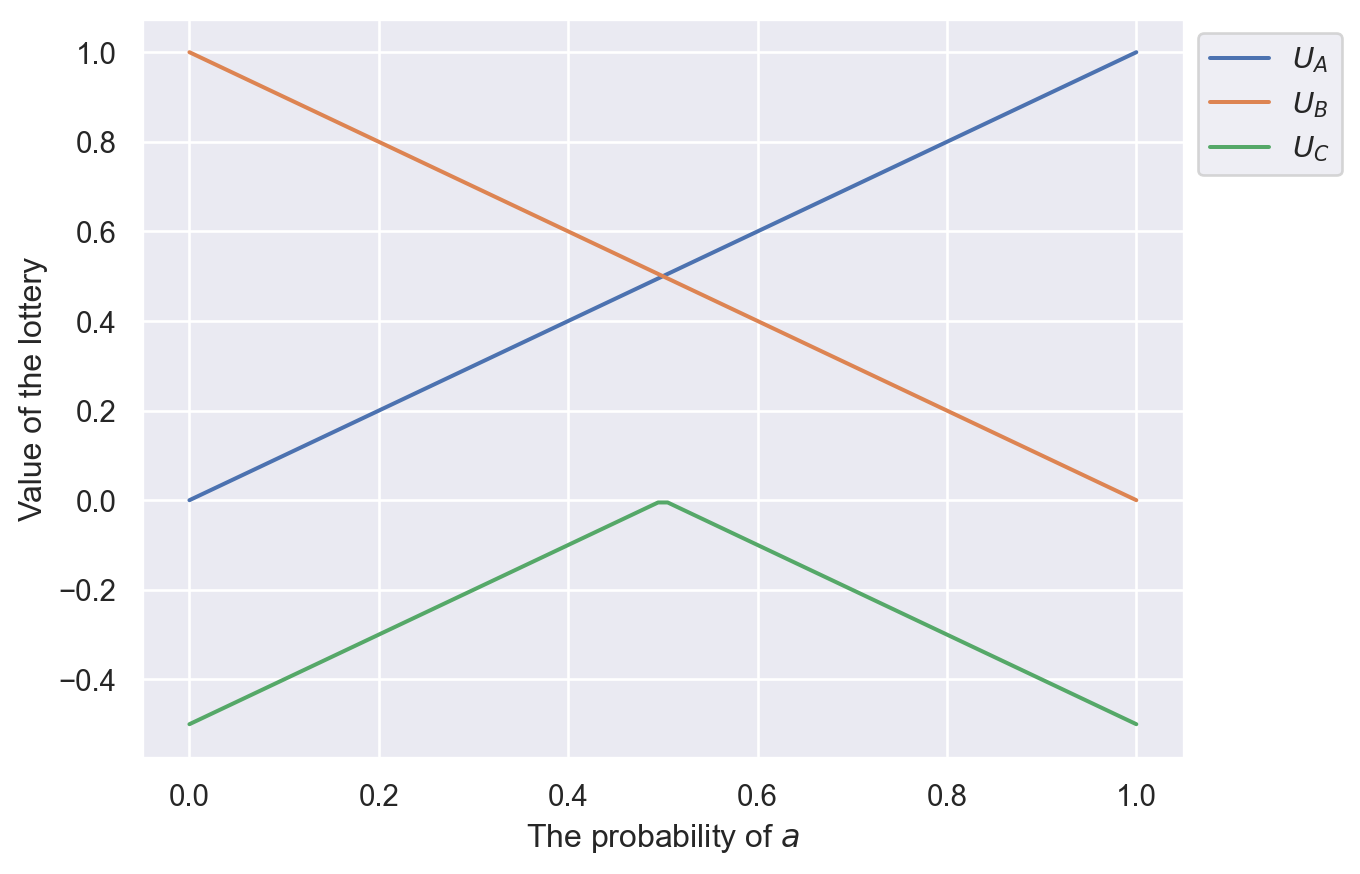
Ann’s utility function is $U_A(r\cdot a + (1-r)\cdot b) = r$, for all $r\in [0, 1]$.
Bob’s utility function is $U_B(r\cdot a + (1-r)\cdot b) = 1-r$, for all $r\in [0, 1]$.
Carol’s utility function is $U_C(r\cdot a + (1-r)\cdot b) = -|r - 0.5|$, for all $r\in [0, 1]$.

Notation for utility functions

In these notes, we use a lowercase “$u$” to represent a utility function on a set $X$, and a capital “$U$” (possibly with subscripts) to represent utility functions on lotteries. This distinction is necessary to differentiate between utility functions on the set $X$ and those on the set $\mathcal{L}(X)$.

The above utility functions are displayed in the following graph:

Figure 11.1: Graphs of the utility functions $U_A$, $U_B$, and $U_C$ as a function of the probability assigned to the outcome $a$.

There is an important difference between Carol’s preferences and those of Ann and Bob over the set of lotteries. Both Ann and Bob’s preferences satisfy the following property:

Definition 11.3 Suppose that $X$ is a finite set, $\mathcal{L}(X)$ is the set of all lotteries over $X$. A rational preference $(P, I)$ over $\mathcal{L}(X)$ is expected utility representable provided that there is a utility function $u:X\rightarrow\mathbb{R}$ such that for all lotteries $L, L'\in\mathcal{L}(X)$,

if $L\mathrel{P} L'$, then $EU(L, u) > EU(L', u)$; and
if $L\mathrel{I} L'$, then $EU(L, u) = EU(L', u)$.

It is straightforward to see that both Ann and Bob’s preferences are expected utility representable (for Ann, consider the utility function that assigns 1 to $a$ and 0 to $b$, and for Bob, consider the utility function that assigns 0 to $a$ and 1 to $b$). In contrast, Carol’s preferences are not expected utility representable.

Explanation why Carol’s preference is not expected utility representable.

Towards a contradiction, suppose that Carol’s preferences are expected utility representable. Then, there is a utility function $u:\{a, b\}\rightarrow\mathbb{R}$ such that

Since $(0.5 \cdot a + 0.5\cdot b) \mathrel{P} (0.75 \cdot a + 0.25\cdot b)$, we have that \[EU(0.5 \cdot a + 0.5\cdot b, u) > EU(0.75 \cdot a + 0.25\cdot b, u).\] This implies that \[\begin{align*} 0.5 \times u(a) + 0.5 \times u(b) &= EU(0.5 \cdot a + 0.5\cdot b, u) \\ &> EU(0.75 \cdot a + 0.25\cdot b, u) \\ &= 0.75 \times u(a) + 0.25 \times u(b) \end{align*}\] Thus, $0.5u(a) + 0.5u(b) > 0.75u(a) + 0.25u(b)$, and so, we have that $u(b) > u(a)$.
Since $(0.75\cdot a + 0.25\cdot b)\mathrel{I}(0.25\cdot a + 0.75\cdot b)$, we have that \[EU(0.75\cdot a + 0.25\cdot b, u) = EU(0.25\cdot a + 0.75\cdot b, u).\] This implies that \[\begin{align*} 0.75\times u(a) + 0.25\times u(b) &= EU(0.75\cdot a + 0.25\cdot b, u) \\ &= EU(0.25\cdot a + 0.75\cdot b, u) \\ &= 0.25 \times u(a) + 0.75 \times u(b) \end{align*}\] Thus, $0.75u(a) + 0.25u(b)= 0.25u(a) + 0.75u(b)$, and so, we have that $u(a) = u(b)$.

Putting 1 and 2 together, we have that $u(b)> u(a) = u(b)$, which is impossible. Thus, Carol’s preferences are not expected utility representable.

To summarize, we note the following three facts about Carol’s preferences over the set of lotteries $\mathcal{L}(\{a, b\})$:

Carol has a rational preference over the set of lotteries $\mathcal{L}(\{a, b\})$.
Carol’s rational preference is representable by the utility function $U_C:\mathcal{L}({a, b})\rightarrow\mathbb{R}$, where for all $r\in [0, 1]$, $U_C(r\cdot a + (1-r)\cdot b) = -|r-0.5|$.
Carol’s rational preference is not expected utility representable.

11.2 Exercises

What is the expected value of $L = 0.2 \cdot \$100 + 0.6 \cdot \$60 + 0.1 \cdot \$0 + 0.1 \cdot \$10$?
What is the expected utility of $L = 0.2 \cdot \$100 + 0.6 \cdot \$60 + 0.1 \cdot \$0 + 0.1 \cdot \$10$ using the utility function where for each monetary amount $m$, $u(m) = \sqrt{m}$?
Suppose that $X = \{a, b, c\}$ and that a rational decision maker strictly prefers $a$ to $b$ and $b$ to $c$. Assuming that the decision maker compares lotteries by comparing their expected utilities, find a utility function on $X$ such that the decision maker strictly prefers $L_2$ to $L_1$, where \[L_1=0.6\cdot a:0.6 + 0.4\cdot c\mbox{ and } L_2 = 1\cdot b\]
Suppose that $X=\{a, b, c\}$ and that a rational decision maker strictly prefers $a$ to $b$ and $b$ to $c$. Assuming that the decision maker compares lotteries by comparing their expected utilities, find a utility function on $X$ such that the decision maker strictly prefers $L_1$ to $L_2$, where \[L_1=0.6\cdot a + 0.4\cdot c\mbox{ and } L_2 = 1\cdot b\]
Suppose that $X=\{a, b, c\}$ and that a rational decision maker strictly prefers $a$ to $b$ and $b$ to $c$. Assuming that the decision maker compares lotteries by comparing their expected utilities, find a utility function on $X$ such that the decision maker is indifferent between the following two lotteries: \[L_1=0.6\cdot a + 0.4\cdot c\mbox{ and } L_2 = 1\cdot b\]
Suppose that Ann is faced with the choice between lotteries $L_1$ and $L_2$ where: \[L_1=0.4\cdot \$4000 + 0.5\cdot \$0\qquad L_2=1\cdot \$3000\] Suppose that Ann ranks $L_2$ over $L_1$ (e.g., $L_2\mathrel{P} L_1$) and that Ann is also faced with the choice between lotteries $L_3$ and $L_4$ where: \[L_3=0.2\cdot\$4000 + 0.8\cdot \$0\qquad L_4=0.5\cdot\$3000 + 0.5\cdot\$0.\] Can we conclude anything about how Ann ranks $L_3$ and $L_4$?
Suppose that a decision maker strictly prefers $a$ to $b$ and $b$ to $c$. Consider the lotteries $L_1 = 0.7 \cdot a + 0.3 \cdot c$ and $L_2 = 0.3 \cdot c + 0.7 \cdot b$. Assuming that the decision maker’s preferences are rational and that she compares lotteries by maximizing expected utility, which of the following is true:
1. The decision maker strictly prefers $L_1$ over $L_2$.
2. The decision maker strictly prefers $L_2$ over $L_1$.
3. The decision maker is indifferent between $L_1$ and $L_2$.
4. There is not enough information to answer this question.

Solutions

What is the expected value of $L=[\$100: 0.2, \$60: 0.6, \$0: 0.1, \$10: 0.1]$?

$EV(L) = 0.2 * 100 + 0.6 * 60 + 0.1 * 0 + 0.1 * 10 = 20 + 3.6 + 0 + 1 = 24.6$
What is the expected utility of $L=[\$100: 0.2, \$60: 0.6, \$0: 0.1, \$10: 0.1]$ using the utility function where for each monetary amount $m$, $u(m)=\sqrt{m}$?

$EU(L, u) = 0.2 * \sqrt{100} + 0.6 * \sqrt{60} + 0.1 * \sqrt{0} + 0.1 * \sqrt{10} =6.964$
Suppose that $X=\{a, b, c\}$ and that a rational decision maker strictly prefers $a$ to $b$ and $b$ to $c$. Assuming that the decision maker compares lotteries by comparing their expected utilities, find a utility function on $X$ such that the decision maker strictly prefers $L_2$ to $L_1$, where \[L_1=[a:0.6, c:0.4]\mbox{ and } L_2 = [b:1].\]

Let $u(a) = 1$, $u(b) =0.7$ and $u(c) = 0$. Then \[EU(L_1, u) = 0.6 * 1 + 0.4 * 0 = 0.6 < EU(L_2, u) = 0.7 * 1 = 0.7\]
Suppose that $X=\{a, b, c\}$ and that a rational decision maker strictly prefers $a$ to $b$ and $b$ to $c$. Assuming that the decision maker compares lotteries by comparing their expected utilities, find a utility function on $X$ such that the decision maker strictly prefers $L_1$ to $L_2$, where \[L_1=[a:0.6, c:0.4]\mbox{ and } L_2 = [b:1].\]

Let $u(a) = 1$, $u(b) =0.5$ and $u(c) = 0$. Then \[EU(L_1, u) = 0.6 * 1 + 0.4 * 0 = 0.6 > EU(L_2, u) = 0.5 * 1 = 0.5\]
Suppose that $X=\{a, b, c\}$ and that a rational decision maker strictly prefers $a$ to $b$ and $b$ to $c$. Assuming that the decision maker compares lotteries by comparing their expected utilities, find a utility function on $X$ such that the decision maker is indifferent between the following two lotteries: \[L_1=[a:0.6, c:0.4]\mbox{ and } L_2 = [b:1]\]

Let $u(a) = 1$, $u(b) =0.6$ and $u(c) = 0$. Then \[EU(L_1, u) = 0.6 * 1 + 0.4 * 0 = 0.6 = EU(L_2, u) = 0.6 * 1 = 0.6\]
Suppose that Ann is faced with the choice between lotteries $L_1$ and $L_2$ where: \[L_1=[\$4000:0.4,\ \$0:0.6]\qquad L_2=[\$3000:1.0]\] Suppose that Ann ranks $L_2$ over $L_1$ (e.g., $L_2\mathrel{P} L_1$) and that Ann is also faced with the choice between lotteries $L_3$ and $L_4$ where: \[L_3=[\$4000:0.2, \$0:0.8]\qquad L_4=[\$3000:0.5, \$0:0.5]\] Can we conclude anything about how Ann ranks $L_3$ and $L_4$?

Ann must rank $L_4$ over $L_3$ (e.g., $L_4\mathrel{P} L_3$).

Suppose that ranks $L_2$ strictly above $L_1$ according to expected utility. Then there is a utility $u: \{\$4000, \$0, \$3000\}\rightarrow \mathbb{R}$ where: \[0.4*u(\$4000) + 0.6*u(\$0) < 1.0* u(\$3000)\]

Then, reason as follows:

\[\begin{align*} 0.4*u(\$4000) + 0.6*u(\$0) &< 1.0* u(\$3000)\\ 0.2*u(\$4000) + 0.3*u(\$0) &< 0.5* u(\$3000) \quad \mbox{(multiply by $0.5$)} \\ 0.2*u(\$4000) + 0.8*u(\$0) &< 0.5* u(\$3000) + 0.5u(\$0) \quad\mbox{(add $0.5*u(\$0)$)} \end{align*}\]

This means that $L_4$ is ranked strictly above $L_3$ according to expected utility theory and Ann’s utility $u: \{\$4000, \$0, \$3000\}\rightarrow \mathbb{R}$.
Suppose that a decision maker strictly prefers $a$ to $b$ and $b$ to $c$. Consider the lotteries $L_1=[a:0.7, c: 0.3]$ and $L_2=[c:0.3, b:0.7]$. Assuming that the decision maker’s preferences are rational and that she compares lotteries by maximizing expected utility, which of the following is true:
1. The decision maker strictly prefers $L_1$ over $L_2$.
2. The decision maker strictly prefers $L_2$ over $L_1$.
3. The decision maker is indifferent between $L_1$ and $L_2$.
4. There is not enough information to answer this question.
Suppose that $u$ is a utility function representing the decision maker’s preferences.

Then $EU(L_1, u) = 0.7u(a) + 0.3u(c)$ and $EU(L_2, u) = 0.3u(c) + 0.7u(b)$

Since $u(a) > u(b)$, we have $0.7u(a) > 0.7u(b)$ and so $0.7u(a) + 0.3u(c) > 0.7u(b) + 0.3u(c)$. Hence, the decision maker must strictly prefer $L_1$ to $L_2$.