12 Expected Utility

12.1 Expected Value

When the prizes are monetary values, a decision maker can compare lotteries using the expected value of the lottery.

Definition 12.1 (Expected value) Suppose that $L=[x_1:p_1, \ldots, x_n:p_n]$ is a lottery where for $i=1, \ldots, n$, $x_i$ is an amount of money. The expected value of $L$ is defined as follows: \[EV(L)=\sum_{i=1}^n p_i * x_i.\]

For example, if $L=[\$100:0.5, \$0:0.5]$, then $EV(L) = 0.5 * 100 + 0.5 * 0 = 50$. This means that you should be willing to pay up to $\$50$ to play this lottery. To illustrate this, you can evaluate the average payout after playing this lottery 1000 times (you can change the probabilities and payouts).

viewof p = Inputs.form({
  prize1: Inputs.range([0, 100], {step: 1, value: 100, label: "prize 1"}),
  prize2: Inputs.range([0, 100], {step: 1, value: 0, label: "prize 2"}),
  prob: Inputs.range([0, 1], {step: 0.01, value:0.5, label: "probability of prize 1"}),
})

tex.block`
  EV([${p.prize1}:${p.prob}, ${p.prize2}: ${Math.round((1-p.prob)*100) / 100}]) = ${p.prob} * ${p.prize1} + ${Math.round((1-p.prob)*100) / 100} * ${p.prize2} = ${Math.round((p.prob * p.prize1 + (1-p.prob) * p.prize2) *1000) / 1000}
`

data_ev={
  let p1_data = {prize: "$" + p.prize1.toString(), num: 0};
  let p2_data = {prize: "$" + p.prize2.toString(), num: 0};
  let x = 0;
  for (let i = 0; i < 1000; i++) {

    let outcome = Math.random() < p.prob ? 1 : 0;
    p1_data["num"] += outcome;
    p2_data["num"] += 1-outcome;
    
}
  return [p1_data, p2_data];
}

md`After playing the lottery 1000 times, the average payout is ${(data_ev[0]["num"] * p.prize1 + data_ev[1]["num"] * p.prize2) / 1000}. The number of times each prize was won is given in the following bar graph: `

Plot.plot({
  marks: [
    Plot.barY(data_ev, {x: "prize", y: "num"})
  ]
})

12.1.1 St. Petersburg Paradox

A problem with evaluating lotteries using their expected value was noticed in the 18th century by the mathematician Nicolas Bernoulli. Bernoulli considered the following lottery: repeatedly flip a coin until it lands heads. If the coin is flipped $n$ times, then the payout is $2^n$. That is, he considered the following lottery:

\[L = [2: \frac{1}{2}, 4: \frac{1}{4}, 16: \frac{1}{16}, \ldots, 2^n: \frac{1}{2^n}, \ldots]\]

Warning

Note that the above lottery uses an infinite set of outcomes.

The problem is that the expected value of this lottery is infinite:

\[EV(L)= \sum_{n=1}^\infty \frac{1}{2^n}*2^n = \sum_{n=1}^\infty 1 = \infty\]

This means that a decision make should be willing to pay any amount of money to play this lottery. One way to avoid this absurd conclusion is to replace the monetary value of an item with its utility, as explained by Daniel Bernoulli in 1738:

the value of an item must not be based on its price, but rather on the utility it yields. The price of the item is dependent only on the thing itself and is equal for everyone; the utility, however, is dependent on the particular circumstances of the person making the estimate. Thus there is no doubt that a gain of one thousand ducats is more significant to a pauper than to a rich man though both gain the same amount.

One way to make the above idea precise is to take the log base $e$ of the prize when calculating the expected value. That is, the value of the lottery $L$ is calculated using the utility rather than payout: \[\sum_{n=1}^\infty\frac{1}{2^n}*\ln(2^n)=\sum_{n=1}^\infty\frac{1}{2^n}*\ln(2^n) < \infty.\]

This solution is illustrated below: The graph lists the number of prizes received after playing the St. Petersburg lottery 1000 times (you can change this value). The table below the graph lists for each number of flips, the probability of observing that flip, the payout, the expected payout, the utility, and the expected payout.

See St. Petersburg Paradox, Stanford Encyclopedia of Philosophy for more discussion about variants and other solutions.

12.2 Expected Utility

Suppose that a decision maker has a lottery ticket that pays $1,000 with probability $0.5$, otherwise it pays nothing. Suppose that the decision maker is offered a chance to trade this lottery ticket for $\$499$. Is it rational for the decision maker to accept this trade? The decision maker is comparing two lotteries: \[L_1 = [1000:0.5, 0:0.5]\quad\mbox{ and }\quad L_2 = [499:1]\] Accepting the trade means that the decision maker revealed a preference of $L_2$ over $L_1$. However, the expected value of $L_1$ is greater than the expected value of $L_2$. Thus, if the decision to trade is rational, then it must be explained using something other than the expected value of the lotteries. As discussed in the previous section, the key idea is to compare lotteries in terms of their expected utilities rather than their expected values.

Definition 12.2 (Expected utility) Suppose that $X$ is a set and $u:X\rightarrow \mathbb{R}$ is a utility function. If $L=[x_1: p_1, \ldots, x_n: p_n]$ is a lottery on $X$. Then, the expected utility of $L$ is: \[EU(L, u) = \sum_{i=1}^n p_i * u(x_i).\]

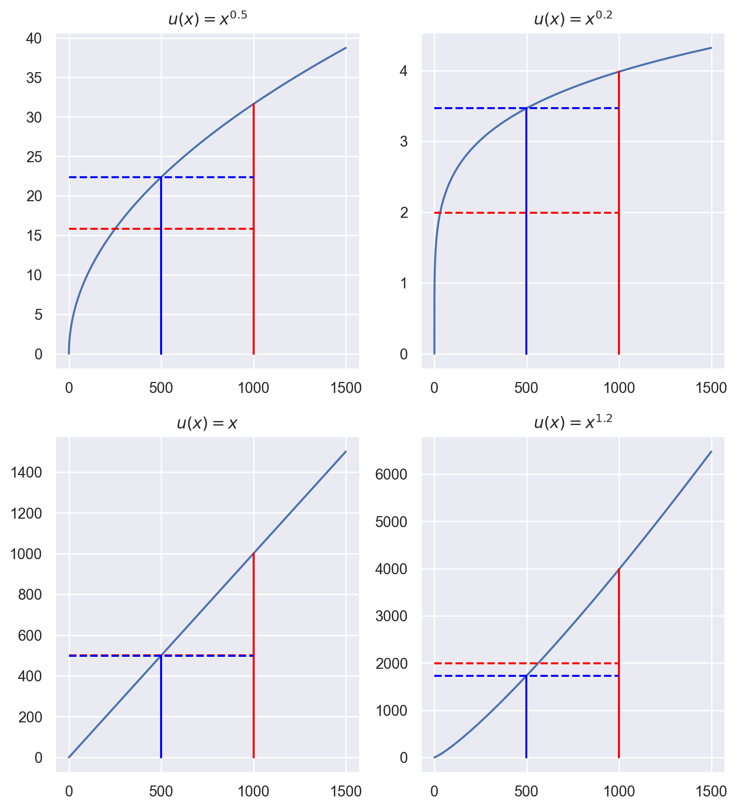
The decision to trade is rational when there is some utility function $u$ on monetary prizes such that $EU(L_2, u) > EU(L_1, u)$. Assuming that $u(\$0) = 0$, then we have that $EU(L_2, u) > EU(L_1, u)$ for any utility function such that $u(499) > 0.5u(1000)$. For instance, if $u(x)=\sqrt(x)$, then \[u(499) = \sqrt{499} = 22.34 > 15.81 = 0.5 \sqrt{1000} = 0.5 * u(1000).\]

One motivation for the above utility function is that the decision maker is risk-averse. That is, the decision maker prefers a sure-thing over a risky lottery even if the sure-thing has a lower expected value. Not all utility function exhibit this type of risk-aversion. For instance, consider the three utility functions depicted in the graphs below. The blue dashed line is $u(499)$ and the red dashed line is $0.5*u(1000)$. The utility functions on the first row are risk-averse, while the utility function on the bottom right represents a decision-maker that is not risk-averse (in fact, this utility function represents a decision maker that is risk-seeking).

12.3 Exercises

What is the expected value of $L=[\$100: 0.2, \$60: 0.6, \$0: 0.1, \$10: 0.1]$?
What is the expected utility of $L=[\$100: 0.2, \$60: 0.6, \$0: 0.1, \$10: 0.1]$ using the utility function where for each monetary amount $m$, $u(m)=\sqrt{m}$?
Suppose that $X=\{a, b, c\}$ and that a rational decision maker strictly prefers $a$ to $b$ and $b$ to $c$. Assuming that the decision maker compares lotteries by comparing their expected utilities, find a utility function on $X$ such that the decision maker strictly prefers $L_2$ to $L_1$, where \[L_1=[a:0.6, c:0.4]\mbox{ and } L_2 = [b:1]\]
Suppose that $X=\{a, b, c\}$ and that a rational decision maker strictly prefers $a$ to $b$ and $b$ to $c$. Assuming that the decision maker compares lotteries by comparing their expected utilities, find a utility function on $X$ such that the decision maker strictly prefers $L_1$ to $L_2$, where \[L_1=[a:0.6, c:0.4]\mbox{ and } L_2 = [b:1]\]
Suppose that $X=\{a, b, c\}$ and that a rational decision maker strictly prefers $a$ to $b$ and $b$ to $c$. Assuming that the decision maker compares lotteries by comparing their expected utilities, find a utility function on $X$ such that the decision maker is indifferent between the following two lotteries: \[L_1=[a:0.6, c:0.4]\mbox{ and } L_2 = [b:1]\]
Suppose that Ann is faced with the choice between lotteries $L_1$ and $L_2$ where: \[L_1=[\$4000:0.4,\ \$0:0.6]\qquad L_2=[\$3000:1.0]\] Suppose that Ann ranks $L_2$ over $L_1$ (e.g., $L_2\mathrel{P} L_1$) and that Ann is also faced with the choice between lotteries $L_3$ and $L_4$ where: \[L_3=[\$4000:0.2, \$0:0.8]\qquad L_4=[\$3000:0.5, \$0:0.5]\] Can we conclude anything about how Ann ranks $L_3$ and $L_4$?
Suppose that a decision maker strictly prefers $a$ to $b$ and $b$ to $c$. Consider the lotteries $L_1=[a:0.7, c: 0.3]$ and $L_2=[c:0.3, b:0.7]$. Assuming that the decision maker’s preferences are rational and that she compares lotteries by maximizing expected utility, which of the following is true:
1. The decision maker strictly prefers $L_1$ over $L_2$.
2. The decision maker strictly prefers $L_2$ over $L_1$.
3. The decision maker is indifferent between $L_1$ and $L_2$.
4. There is not enough information to answer this question.

Solutions

What is the expected value of $L=[\$100: 0.2, \$60: 0.6, \$0: 0.1, \$10: 0.1]$?

$EV(L) = 0.2 * 100 + 0.6 * 60 + 0.1 * 0 + 0.1 * 10 = 20 + 3.6 + 0 + 1 = 24.6$
What is the expected utility of $L=[\$100: 0.2, \$60: 0.6, \$0: 0.1, \$10: 0.1]$ using the utility function where for each monetary amount $m$, $u(m)=\sqrt{m}$?

$EU(L, u) = 0.2 * \sqrt{100} + 0.6 * \sqrt{60} + 0.1 * \sqrt{0} + 0.1 * \sqrt{10} =6.964$
Suppose that $X=\{a, b, c\}$ and that a rational decision maker strictly prefers $a$ to $b$ and $b$ to $c$. Assuming that the decision maker compares lotteries by comparing their expected utilities, find a utility function on $X$ such that the decision maker strictly prefers $L_2$ to $L_1$, where \[L_1=[a:0.6, c:0.4]\mbox{ and } L_2 = [b:1].\]

Let $u(a) = 1$, $u(b) =0.7$ and $u(c) = 0$. Then \[EU(L_1, u) = 0.6 * 1 + 0.4 * 0 = 0.6 < EU(L_2, u) = 0.7 * 1 = 0.7\]
Suppose that $X=\{a, b, c\}$ and that a rational decision maker strictly prefers $a$ to $b$ and $b$ to $c$. Assuming that the decision maker compares lotteries by comparing their expected utilities, find a utility function on $X$ such that the decision maker strictly prefers $L_1$ to $L_2$, where \[L_1=[a:0.6, c:0.4]\mbox{ and } L_2 = [b:1].\]

Let $u(a) = 1$, $u(b) =0.5$ and $u(c) = 0$. Then \[EU(L_1, u) = 0.6 * 1 + 0.4 * 0 = 0.6 > EU(L_2, u) = 0.5 * 1 = 0.5\]
Suppose that $X=\{a, b, c\}$ and that a rational decision maker strictly prefers $a$ to $b$ and $b$ to $c$. Assuming that the decision maker compares lotteries by comparing their expected utilities, find a utility function on $X$ such that the decision maker is indifferent between the following two lotteries: \[L_1=[a:0.6, c:0.4]\mbox{ and } L_2 = [b:1]\]

Let $u(a) = 1$, $u(b) =0.6$ and $u(c) = 0$. Then \[EU(L_1, u) = 0.6 * 1 + 0.4 * 0 = 0.6 = EU(L_2, u) = 0.6 * 1 = 0.6\]
Suppose that Ann is faced with the choice between lotteries $L_1$ and $L_2$ where: \[L_1=[\$4000:0.4,\ \$0:0.6]\qquad L_2=[\$3000:1.0]\] Suppose that Ann ranks $L_2$ over $L_1$ (e.g., $L_2\mathrel{P} L_1$) and that Ann is also faced with the choice between lotteries $L_3$ and $L_4$ where: \[L_3=[\$4000:0.2, \$0:0.8]\qquad L_4=[\$3000:0.5, \$0:0.5]\] Can we conclude anything about how Ann ranks $L_3$ and $L_4$?

Ann must rank $L_4$ over $L_3$ (e.g., $L_4\mathrel{P} L_3$).

Suppose that ranks $L_2$ strictly above $L_1$ according to expected utility. Then there is a utility $u: \{\$4000, \$0, \$3000\}\rightarrow \mathbb{R}$ where: \[0.4*u(\$4000) + 0.6*u(\$0) < 1.0* u(\$3000)\]

Then, reason as follows:

\[\begin{align*} 0.4*u(\$4000) + 0.6*u(\$0) &< 1.0* u(\$3000)\\ 0.2*u(\$4000) + 0.3*u(\$0) &< 0.5* u(\$3000) \quad \mbox{(multiply by $0.5$)} \\ 0.2*u(\$4000) + 0.8*u(\$0) &< 0.5* u(\$3000) + 0.5u(\$0) \quad\mbox{(add $0.5*u(\$0)$)} \end{align*}\]

This means that $L_4$ is ranked strictly above $L_3$ according to expected utility theory and Ann’s utility $u: \{\$4000, \$0, \$3000\}\rightarrow \mathbb{R}$.
Suppose that a decision maker strictly prefers $a$ to $b$ and $b$ to $c$. Consider the lotteries $L_1=[a:0.7, c: 0.3]$ and $L_2=[c:0.3, b:0.7]$. Assuming that the decision maker’s preferences are rational and that she compares lotteries by maximizing expected utility, which of the following is true:
1. The decision maker strictly prefers $L_1$ over $L_2$.
2. The decision maker strictly prefers $L_2$ over $L_1$.
3. The decision maker is indifferent between $L_1$ and $L_2$.
4. There is not enough information to answer this question.
Suppose that $u$ is a utility function representing the decision maker’s preferences.

Then $EU(L_1, u) = 0.7u(a) + 0.3u(c)$ and $EU(L_2, u) = 0.3u(c) + 0.7u(b)$

Since $u(a) > u(b)$, we have $0.7u(a) > 0.7u(b)$ and so $0.7u(a) + 0.3u(c) > 0.7u(b) + 0.3u(c)$. Hence, the decision maker must strictly prefer $L_1$ to $L_2$.